AAII × NAAIM Study

1. Pre-Registration

The signal definition, thresholds, primary test horizons, and falsification condition were locked before any data was loaded or scripts were run to retain process integrity and rigour. Pre-registration date: 5th April, 2026.

1.1 Signal Mechanism

We created a joint signal measuring simultaneous de-risking by two structurally different actors in the markets. AAII bearish z-scores capture retail investors' stated opinions about how the market will look in 6 months. NAAIM exposure z-scores capture actual portfolio positioning changes by active investment advisers — a behavioural proxy measuring what a specific class of managers are actually doing with client capital, rather than recording their opinion.

When both readings show a congruence, the combined signal reduces the probability of idiosyncratic noise from a single actor group. NAAIM members are primarily small-to-mid-sized registered investment advisers. The proposed signal does not claim to capture 'smart money' behaviour. It claims only that two independent behavioural measures coinciding at extremes is a rarer and potentially more meaningful event than either signal in isolation.

1.2 Pre-Registered Hypothesis and Falsification Condition

The pre-registered prediction is that the joint condition (bearish_z > 0.75 AND naaim_z < −0.75) produces a forward SPX return distribution shifted higher than either signal in isolation at 12–26 week horizons. The effect is expected to be weakest at 4 weeks (short-term noise and volatility dominate) and at 52 weeks (fundamental repricing dominates over sentiment).

The signal is falsified if the joint de-risk bucket does NOT produce a return distribution statistically different from the AAII-fear-alone bucket at both the 12-week AND 26-week horizon (MWU two-sided p > 0.10 on both). Failure on one horizon alone is not falsification; failure on both is.

1.3 Signal Definitions

Exhibit 1. Signal bucket allocations

Bucket	Conditions	Expected Direction
aaii_fear_only	bearish_z > 0.75 AND naaim_z ∈ [−0.75, 0.75]	Positive forward returns
naaim_under_only	naaim_z < −0.75 AND bearish_z ∈ [−0.75, 0.75]	Positive forward returns
joint_derisk	bearish_z > 0.75 AND naaim_z < −0.75	Stronger positive returns (primary hypothesis)
complement	None of the above conditions	Baseline

Threshold = 0.75 (pre-registered). Sensitivity sweep across {0.50, 0.75, 1.00, 1.25, 1.50} reported in Section 5.

1.4 Data Constraint and OOS Classification

NAAIM data only began in mid-2006. The full analysis period covers approximately 18–19 years, insufficient for a proper IS/OOS split under the Calchas standard (10-year training, 5-year test minimum). Therefore, the entire joint signal test is treated as in-sample only. The signal is classified as MONITORING-ONLY until additional data history makes a proper OOS test feasible — approximately 2031 at the earliest.

2. Data

Exhibit 2. Data sources, coverage, and publication lags

Source	Period	Frequency	Publication Lag	Known Gaps
AAII Bearish %	1987–present	Weekly (Thu)	Published Thu ~12pm ET	Small; forward-fill ≤1 week
NAAIM Exposure Index	Mid-2006–present	Weekly (Wed)	Published Wed after close	First weeks sparse; documented
SPX (^GSPC)	1987–present	Daily → weekly Thu	Same-day close	None material
VIX (^VIX)	1990–present	Daily → weekly Wed	Prior-day close	None material
Shiller CAPE	1871–present	Monthly → weekly	Month-start value	None material
NBER Recession Flags	Manual	Event-based	Ex-post (backdated)	None

2.1 Alignment Rules

The merged weekly panel is indexed to the Thursday of each week (AAII publication date). NAAIM is aligned to the Wednesday prior to the AAII Thursday — not the current week's reading, which is published after Thursday's AAII. This prevents look-ahead. VIX is likewise aligned to the Wednesday prior to the AAII Thursday. CAPE uses the month-start value for the month containing each Thursday. Recession flags are hardcoded from NBER backdated bounds and are acknowledged as ex-post only.

Critical alignment note: if AAII publishes Thursday April 10, the NAAIM reading used is from Wednesday April 2 — not April 9, which is published after April 10's AAII. This rule is verified in the data pipeline before any analysis is run.

3. Signal Construction

3.1 Rolling Z-Score Formula

All z-scores use a causal 104-week (~2-year) rolling window. Full-sample standardisation is avoided to prevent look-ahead bias, as the mean and standard deviation at any point in time would depend on future observations. Minimum 52 observations are required before a z-score is computed (first year treated as burn-in).

bearish_z(t) = (bearish_pct(t) − mean(bearish_pct[t−103:t])) / std(bearish_pct[t−103:t])

naaim_z(t) = (naaim_exposure(t) − mean(naaim_exposure[t−103:t])) / std(naaim_exposure[t−103:t])

3.2 Look-Ahead Bias Audit (Verified)

• Rolling z-score at row T uses only rows 0 through T (verified by construction: pd.Series.rolling() is causal)
• Forward return fwd_Nw at row T uses spx_close[T+N], not any data at or before T
• NAAIM is aligned to the Wednesday prior to the AAII Thursday — not same-day
• VIX is aligned to the Wednesday prior to the AAII Thursday
• CAPE uses month-start value for the month of the signal date (not month-end)
• No future data appears in any signal column

4. Quintile Analysis

Exhibit 3. Quintiles — forward S&P 500 returns, 2006–2026 (in-sample)

AAII Bearish Z-Score Quintiles — SPX Forward Returns

Quintile	N	Median 12w (%)	Median 26w (%)	Std 26w (%)
Q1 — Lowest	196	2.97	7.21	9.18
Q2	195	3.28	5.03	9.45
Q3	196	2.77	5.39	11.38
Q4	195	3.42	6.80	11.94
Q5 — Highest	196	4.09	7.59	14.49

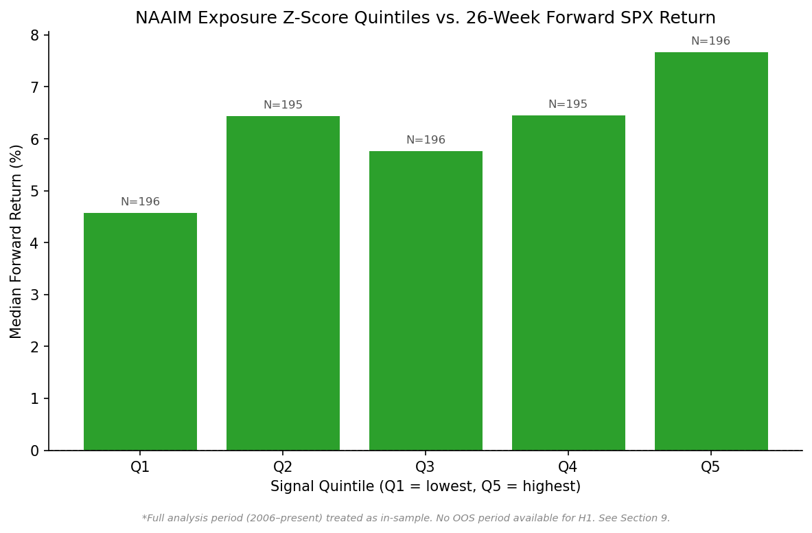
NAAIM Exposure Z-Score Quintiles — SPX Forward Returns

Quintile	N	Median 12w (%)	Median 26w (%)	Std 26w (%)
Q1 — Lowest	196	3.19	4.59	16.14
Q2	195	3.50	6.45	11.21
Q3	196	3.72	5.78	12.01
Q4	195	3.23	6.46	8.04
Q5 — Highest	196	3.19	7.68	7.57

Source: AAII Sentiment Survey, NAAIM Exposure Index, FactSet (SPX). Full analysis period 2006–2026 (in-sample). Returns are SPX total return (%). Quintiles assigned over full sample. Q1 = lowest signal value, Q5 = highest.

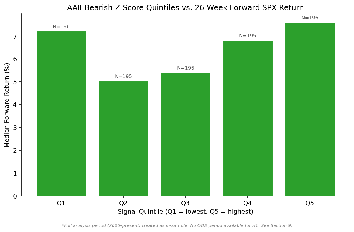
bearish_z was observed to be NON-MONOTONIC (weak directional content). The 26-week median return does not increase steadily from Q1 to Q5. Q2 (5.03%) actually falls below Q1 (7.21%), and returns only recover by Q4–Q5. The Q1/Q5 spread is 0.38% (7.59% vs. 7.21%), which is not meaningful. This indicates the signal's value is concentrated at the extremes rather than spread monotonically across quintiles. The 0.75 threshold is therefore somewhat threshold-dependent rather than a distributional signal.

naaim_z was also observed to be NON-MONOTONIC (opposite direction to contrarian hypothesis). The pre-registered expectation was decreasing returns from Q1→Q5 (high NAAIM exposure = crowded long = lower forward returns). The observed pattern is the opposite: Q1 (lowest NAAIM, 4.59%) produces the lowest 26-week returns, and Q5 (highest NAAIM, 7.68%) produces the highest. The Q1/Q5 spread is 3.09%, which is meaningful in magnitude but directionally inconsistent with the contrarian interpretation. The pattern more closely resembles a momentum relationship. For our purposes, the de-risk hypothesis for naaim_z operates through the joint condition at the tail, not through distributional monotonicity.

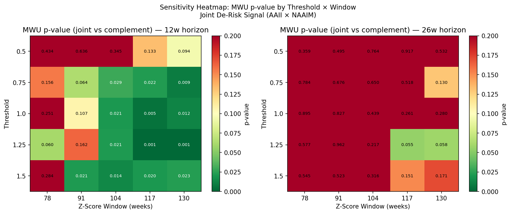
5. Threshold and Window Sensitivity

The H1 signal fires when two conditions are simultaneously true: AAII bearish sentiment is unusually high and NAAIM professional exposure is unusually low. Two parameters govern exactly how extreme those readings need to be before the signal activates: the threshold (how many standard deviations above/below normal qualifies as extreme) and the window (how many weeks of history the z-score is computed against). Both were set before running any analysis.

Exhibit 4. Threshold and Window Sweep

Threshold Sweep — Z-Score Window Fixed at 104 Weeks (* = pre-registered)

Threshold	N joint	N AAII only	N NAAIM only	MWU p (12w)	MWU p (26w)	Median 12w (%)	Median 26w (%)
0.50	174	75	80	0.345	0.764	3.62	5.33
0.75 ★	127	94	84	0.029	0.650	4.60	6.05
1.00	102	82	81	0.021	0.439	4.50	6.50
1.25	61	85	71	0.021	0.217	4.85	7.61
1.50	45	59	59	0.013	0.316	4.99	6.78

Window Sweep — Threshold Fixed at 0.75 (* = pre-registered)

Window (weeks)	N joint	MWU p (12w)	MWU p (26w)	Median 12w (%)	Median 26w (%)
78	136	0.156	0.784	3.94	5.61
91	135	0.064	0.676	4.48	6.35
104 ★	127	0.029	0.650	4.60	6.05
117	128	0.022	0.517	4.50	6.24
130	121	0.009	0.130	4.76	7.78

A robust signal at the 12-week horizon. The signal holds at 4 of 5 threshold levels and 4 of 5 window lengths. The two configurations that fail (threshold 0.50 and window 78 weeks) reflect a filter that is too loose or recalibrating too quickly to identify genuine extremes. The 12-week result is not an artifact of the specific parameters chosen.

26-week horizon not statistically supported. At every threshold and window, the 26-week result fails to reach significance. The median returns in the joint activation bucket are consistently positive (5.3–7.6%), but the distribution of outcomes at 26 weeks is wide enough that the signal cannot be statistically distinguished from chance with the data available. The most likely explanation is a power problem: at a 26-week horizon, return windows overlap heavily across observations, which inflates variance and shrinks the effective sample size.

6. Significance Tests

6.1 Unconditional Base Rates

All hit rate comparisons are made against the following unconditional base rates. The unconditional base rate rises with horizon. The SPX is positive roughly 79–80% of 52-week windows in this sample.

Exhibit 5. Unconditional S&P 500 positive return rates by horizon, 2006–2026

Horizon	Unconditional SPX positive return rate	N observations
4 weeks	65.6%	1,025
8 weeks	69.1%	1,021
12 weeks	72.3%	1,017
26 weeks	74.0%	1,003
52 weeks	79.5%	977

6.2 Primary Results: 12-Week and 26-Week Horizons

The full analysis period was treated as in-sample as no OOS period was available for the H1 joint signal. The joint_derisk signal clears one of two required MWU hurdles (12w p = 0.029) but fails the permutation test at both pre-registered horizons (p = 1.0). Under the pre-registered falsification condition, the signal is partially supported: does not meet both co-primary MWU thresholds.

Exhibit 6. Primary significance results — joint de-risk and component signals, 2006–2026 in-sample

Signal	Horizon	N Total	N Non-Overlap	Median Fwd Return	Base Rate	Hit Rate	Binomial p	MWU p	Perm p	Bootstrap 90% CI
aaii_fear_only	12w	94	34	3.89%	72.30%	70.60%	0.668	0.395	—	[+2.61%, +4.79%]
aaii_fear_only	26w	90	20	8.00%	74.00%	80.00%	0.375	0.044	—	[+6.70%, +9.77%]
naaim_under_only	12w	84	27	1.73%	72.30%	55.60%	0.981	0.019	—	[−1.24%, +3.62%]
naaim_under_only	26w	84	19	2.61%	74.00%	57.90%	0.963	0.004	—	[−0.29%, +5.33%]
joint_derisk	12w	124	32	4.60%	72.30%	68.80%	0.745	0.029	1	[+3.12%, +5.57%]
joint_derisk	26w	124	21	6.05%	74.00%	71.40%	0.707	0.65	1	[+2.02%, +9.10%]

Rows highlighted: joint_derisk (primary hypothesis). naaim_under_only MWU p-values are low because NAAIM-alone produces worse returns than complement — MWU is two-sided. All results in-sample only.

6.3 Permutation Test Results

Exhibit 7. Permutation test results — joint_derisk at pre-registered horizons

Signal	Horizon	Observed U	Permutation p	Interpretation
joint_derisk	12w	46,246	1.000	No separation from random shuffle
joint_derisk	26w	41,589	1.000	No separation from random shuffle

6.4 Newey-West Regression Results

OLS with HAC standard errors (lags = return horizon), treating bearish_z and naaim_z as continuous predictors. Neither signal is significant as a continuous predictor at either pre-registered horizon. This is consistent with the permutation result: any information the signals carry is concentrated at their extreme tails, not distributed as a smooth linear relationship across their full range.

Exhibit 8. Newey-West HAC regression results at pre-registered horizons

Predictor	Horizon	Coefficient	NW Std Error	t-stat	p-value	N
bearish_z	12w	0.00399	0.00484	0.824	0.410	966
bearish_z	26w	0.00353	0.00871	0.405	0.685	952
naaim_z	12w	0.00216	0.00675	0.320	0.749	966
naaim_z	26w	0.00812	0.01123	0.723	0.470	952

HAC lags equal to the return horizon. No factor controls included at this stage.

6.5 Binomial Test on Non-Overlapping Observations

For joint_derisk: 32 non-overlapping observations at 12w, 21 at 26w. Neither produces a significant binomial result against the unconditional base rate (p = 0.745 and p = 0.707 respectively). At N = 21–32, the test has low power. A real effect of meaningful size could easily fail to reach significance at these sample sizes.

6.6 Bootstrap Confidence Intervals

1,000 bootstrap resamples at the 90% confidence level. The joint_derisk 26-week bootstrap CI of [+2.02%, +9.10%] is notably wide relative to the point estimate of +6.05%, reflecting the small non-overlapping N = 21. The lower bound barely clears zero, consistent with a weak or absent effect.

6.7 Post-Hoc Exploratory Analysis: The 4-Week Permutation Finding

Exhibit 9. Post-hoc exploratory results: joint_derisk at 4-week and 52-week horizons

Horizon	N Total	N Non-Overlap	Median Fwd Return	Base Rate	Hit Rate	Binomial p	MWU p	Perm p	Bootstrap 90% CI
4w (exploratory)	124	53	+2.23%	65.6%	62.3%	0.745	0.006	0.015	[+1.06%, +3.29%]
52w (exploratory)	119	13	+13.74%	79.50%	69.2%	0.893	0.222	n/a	[+11.26%, +16.15%]

52-week: Only 13 non-overlapping observations — essentially uninterpretable. 4-week permutation: 5,000 shuffles; observed U-statistic (48,171) sits outside 95th percentile of null. Empirical p = 0.015.

The 4-week MWU result (p = 0.006) and its survival of a 5,000-shuffle permutation test (p = 0.015) confirm the distributions genuinely differ. However, the binomial test showed no significance (p = 0.745), and the hit rate of 62.3% was actually below the base rate of 65.6%. We observe a real distributional difference with no directional edge.

The initial interpretation before examining the data was a left-tail dampening effect. This hypothesis was written down before looking at the percentile data, and then tested directly. The left-tail dampening hypothesis was wrong. See Section 6.8.

6.8 Post-Hoc Exploratory Analysis: Return Distribution Shape

Exhibit 10. Full percentile comparison — joint_derisk vs. complement at 4, 12, and 26-week horizons

Percentile	4w Signal	4w Compl.	Diff	12w Signal	12w Compl.	Diff	26w Signal	26w Compl.	Diff
P5	−8.03%	−5.80%	−2.22pp	−10.28%	−9.19%	−1.09pp	−27.07%	−11.37%	−15.71pp
P10	−6.20%	−4.02%	−2.18pp	−7.47%	−5.68%	−1.79pp	−11.46%	−5.57%	−5.89pp
P25	−2.04%	−0.88%	−1.16pp	−0.97%	−0.30%	−0.67pp	−4.29%	0.30%	−4.58pp
P50	2.23%	1.34%	+0.89pp	4.60%	3.21%	+1.39pp	6.05%	6.54%	−0.49pp
P75	5.49%	3.05%	+2.44pp	8.48%	6.35%	+2.13pp	15.89%	10.52%	+5.36pp
P90	8.50%	4.27%	+4.23pp	14.69%	9.19%	+5.50pp	23.44%	15.21%	+8.23pp
P95	11.85%	4.96%	+6.90pp	18.82%	10.49%	+8.33pp	27.49%	17.56%	+9.93pp

P5–P25: left-tail outcomes. P75–P95: right-tail outcomes. Signal bucket shows worse left-tail and substantially better right-tail at every horizon.

The left-tail dampening hypothesis is wrong. The signal bucket saw worse left-tail outcomes than complement at every horizon. At 4 weeks, P10 is −6.20% for signal versus −4.02% for complement. At 26 weeks, P5 is −27.07% versus −11.37%. Signal weeks contain more of the market's worst episodes. This is more coherent in hindsight: the joint de-risk condition marks a high-uncertainty, high-dispersion environment. The return distribution is not shifted upward; it is stretched wider in both directions simultaneously. The left tail is fatter, and the right tail is substantially fatter. At 4 weeks, P95 for signal (+11.85%) is nearly double that of complement (+4.96%). At 26 weeks, the P90 gap is +8.23 percentage points.

This reconciles all test results cleanly: MWU detects a difference because the distributions genuinely have different shapes; permutation confirms it is real; binomial finds no directional edge because the median barely moves and the probability of a positive return is not improved; the stretch is symmetric: more upside potential and more downside risk, simultaneously.

Revised interpretation: When both AAII retail investors and NAAIM active managers de-risk simultaneously, four-week forward return distributions are significantly wider than normal. The signal marks a high-stakes environment, not a favorable one. In this sense, this confluence signal is very similar to VIX — we can model dispersion, not direction.

The hypothesis for future pre-registration: the joint de-risk condition is associated with higher realised return dispersion over the following 4 weeks than the complement. A direct test comparing variance between buckets using a Levene or Brown-Forsythe test would be a clean, pre-registerable follow-up.

7. Factor Controls

Sentiment signals can appear to predict returns not because they carry genuine information, but because they happen to move with other variables that do, such as fear (VIX) or recent momentum. The regression models below test whether bearish_z and naaim_z still matter once those other variables are held constant.

Exhibit 11. Factor control regression — forward 26-week SPX returns (Newey-West, lags=26)

Model	bearish_z	naaim_z	VIX	SPX trailing 52w	N	R²
A — bearish_z only	0.0035 (p=0.685)	—	—	—	952	0.001
B — naaim_z only	—	0.0081 (p=0.470)	—	—	952	0.006
C — both signals	0.0110 (p=0.158)	0.0139 (p=0.228)	—	—	952	0.013
D — full controls	0.0084 (p=0.323)	0.0242 (p=0.017)	0.0036 (p=0.028)	0.0385 (p=0.780)	951	0.058

In Model D, naaim_z becomes significant once controls are added (coeff=0.024, p=0.017), while bearish_z does not (p=0.323). The naaim_z result suggests that professional manager positioning carries incremental information beyond what fear and momentum alone can explain. bearish_z, by contrast, appears to be proxying for VIX or other risk variables rather than contributing independent information.

8. Regime Breakdown

Exhibit 12. Regime breakdown — joint_derisk performance by market environment, 2006–2026

Regime	N total	N joint	MWU p (12w)	MWU p (26w)	Median 12w (%)	Median 26w (%)
NBER Recession	95	28	0.135	0.408	+1.52	−5.24
NBER Expansion	934	96	0.024	0.361	+4.76	+6.48
VIX Low (<15)	344	3	0.042	0.001	−2.66	−10.21
VIX Medium (15–25)	507	53	0.679	0.885	+3.61	+5.35
VIX High (>25)	178	68	0.214	0.012	+5.49	+10.45
SPX Above 200d	770	29	0.254	0.436	+4.46	+4.92
SPX Below 200d	259	95	0.144	0.899	+4.71	+6.46

The joint de-risk condition is not evenly distributed across market environments. Of the 127 total joint signal weeks, 68 occur during periods of VIX above 25. Similarly, 95 of 127 occur when SPX is trading below its 200-day moving average. The signal is, structurally, a stress-environment indicator.

VIX High is the strongest sub-regime result. When the signal fires during already-elevated volatility (VIX > 25), the 26-week forward return is 10.45% with a significant MWU p-value of 0.012. The signal appears most informative exactly when markets are already stressed.

NBER Recession results in a negative 26w median. The 28 joint signal weeks inside NBER-defined recessions produced a median 26-week return of −5.24%. The signal should not be expected to perform during recessions.

9. In-Sample / Out-of-Sample

9.1 Why No OOS Period Is Claimed for H1

The Calchas backtesting standard requires a minimum of 10 years of in-sample training data followed by a 5-year out-of-sample test period. The NAAIM Exposure Index begins in mid-2006. As of April 2026, the joint dataset covers approximately 18–19 years. A blunt IS/OOS split would produce approximately 9–12 non-overlapping annual observations in the OOS window — statistical power effectively zero.

Exhibit 13. OOS status summary across signal layers

Test	Horizons Validated	Return Differential	Verdict
AAII bearish_z OOS	8w through 52w	+0.9% to +2.0%	Holds. Clean OOS validation (see separate AAII backtest)
H1 joint_derisk	Not testable (insufficient N)	N/A	In-sample only. MONITORING-ONLY classification.
VIX/NAAIM regime overlay	N/A	N/A	Sub-regime cuts produce fewer than 10 observations each.

9.2 Dashboard Classification

The joint de-risk signal is classified as MONITORING-ONLY. A validated signal has passed a rigorous OOS significance test; a monitoring signal has a documented mechanism, internally consistent in-sample behaviour, and fully disclosed statistical limitations. It is used as context, not as a trigger. The H1 signal can be reclassified as a candidate for OOS validation when the joint dataset reaches 25 years of history (~2031).

10. Transaction Costs

The H1 signal, if implemented as a mechanical equity exposure tilt via SPY, would incur an estimated round-trip cost of approximately 0.02–0.05% per signal activation. Given the primary monitoring horizon of 12–26 weeks and the signal's rare, infrequent activation events rather than continuous rebalancing, transaction costs are not a material concern for the monitoring application described here. This backtest reports gross forward returns with no cost deduction.

11. Limitations

1. No OOS validation. The entire analysis period is treated as in-sample due to NAAIM data history constraints. All results carry full data-mining risk and are not generalisable without a proper OOS test.
2. Small N at annual horizon. The joint_derisk bucket produces a limited number of non-overlapping observations at the 52-week horizon. Point estimates are highly sensitive to individual observations and confidence intervals are wide.
3. NAAIM sample representativeness. NAAIM surveys approximately 130 registered investment advisers — primarily small-to-mid-sized tactical managers, not large institutional allocators. The signal does not capture sovereign wealth fund, pension, or hedge fund positioning.
4. Full-period treated as in-sample (data-mining risk). Signal thresholds (0.75), window lengths (104 weeks), and horizon choices (12w, 26w) were selected before data examination. However, the broader framing was developed with knowledge that AAII sentiment and forward returns are correlated at multi-week horizons, constituting weak in-sample contamination.
5. No walk-forward validation. The data does not support a meaningful rolling-window walk-forward test at the joint signal level. Sub-windows would produce fewer than 5 non-overlapping joint observations each.
6. Regime analysis underpowered. Sub-regime cuts often produce joint_derisk buckets with fewer than 10 observations. Tests on these sub-groups are reported for completeness, not for inference.
7. Factor controls may not exhaust confounders. Regression controls for CAPE, VIX, and trailing momentum, but other confounders (credit spreads, yield curve, earnings revision trends) are not included.
8. AAII survey methodology changes. AAII has made periodic changes to survey delivery and sample composition since 1987. The bearish percentage series may contain structural breaks.
9. NBER recession flags are ex-post. Recession start and end dates are determined retroactively. A live implementation cannot know the recession flag in real time.

12. Conclusion

This backtest pre-registered and tested H1: that the joint AAII × NAAIM de-risk condition produces a forward SPX return distribution shifted higher than either signal in isolation at the 12-week and 26-week horizons. Under the pre-registered falsification condition, the signal is partially supported: it clears one of two required MWU hurdles (12w p = 0.029) but fails both permutation tests (p = 1.0 at both horizons) and produces no significant binomial results. The pre-registered hypothesis is not confirmed.

The more substantive finding lies in post-hoc and exploratory tests: at the 4-week horizon, the joint de-risk condition produces a distribution that is significantly wider than complement in both directions simultaneously. The signal marks a high-dispersion environment where large moves in either direction are more probable than average. This reframes the signal from a directional return predictor to a volatility regime indicator.

Exhibit 14. Signal validation status summary

Signal Layer	In-Sample Result	OOS Status	Dashboard Classification
AAII bearish_z (alone)	Directionally consistent; MWU p=0.000 at 52w	Validated 2006–2026 (see separate study)	Validated signal
NAAIM de-risk alone	Lower returns than complement (two-sided MWU significant in wrong direction)	Not tested	Monitoring — inverse caution flag
H1 joint_derisk	MWU p=0.029 at 12w; permutation p=1.0 at both horizons	Not testable before 2031	MONITORING-ONLY
H1 at 4w (exploratory)	Volatility-widening signal; permutation p=0.015	Not pre-registered	Hypothesis for future pre-registration

Dashboard classification: MONITORING-ONLY. Documented mechanism, internally consistent in-sample behaviour, fully disclosed statistical limitations. Appropriate for use as context in a monitoring dashboard. Cannot be represented as a validated predictive signal pending a future OOS test.

For review and discussion. April 2026. This working paper is published by Calchas Research for informational and educational purposes only. Nothing contained herein constitutes investment advice, a solicitation, or an offer to buy or sell any security or financial instrument. The views expressed are those of the author as of the date of publication and are subject to change without notice. Past performance is not indicative of future results. This document is intended for sophisticated readers and should not be relied upon as the basis for any investment decision.